How to use Excel Indirect function(7 examples, with reference another sheet,extract data in batches)

The Indirect function is used to return a reference to a cell specified by a text string in Excel. There are two types of reference, one for A1-styles and the other for R1C1-styles, which are set by logical values true or false. The cells to be referenced can be the same table, or the same document or cross-document, the latter two cases are cross-table references.

Indirect functions are often used in combination with the Address, Row, Column, and Match functions. For example, the Indirect + Row + Address + Column function combination extracts the specified data of row from multiple tables into a table; the Indirect + Match + Column function combination extracts data in batches by criteria.

I, The syntax of the Excel Indirect function

1. Expression: INDIRECT(Ref_Text,[A1])

2. Description:

A. Ref_Text can be either an internal reference(referenced in this workbook, that is, referenced in the same Sheet or referenced to another Sheet in a Sheet) or an external reference(a reference to another workbook, ie in a document reference another document); It is worth noting that when an external reference is made, the referenced workbook must be opened, otherwise the Indirect function will return a reference error #Ref!. In addition, Excel Web App does not support external references.

B. If the range referenced by Ref_Text exceeds the maximum number of rows 1048576 allowed by Excel or the maximum number of columns 16384(XFD), the Indirect function also returns a reference error #REF!; however, earlier versions of Excel ignored this limit and returned a value.

C. A1 has two optional values, which are True(or omitted) and False; if True, it is interpreted as an A1-style reference; if False, it is interpreted as an R1C1-style reference, and R means "row", C means "column", and R1C1 means a reference to the cell at the intersection of the first row and the first column, that is, A1. Regardless of the reference method, the Indirect function will return an error if the cell to be  referenced does not exist.

II, The examples of Excel Indirect function

(I) How to use indirect in excel(Type of Reference A1 is True(or omitted))

1. Select the cell A9, enter the formula =Indirect(B5), press Enter, return the reference error #REF!; double-click B9, copy the formula =INDIRECT("B"&5) to B9, press Enter, return to the name "Fulinter" in B5; double-click B9, enter ",true" after 5, press Enter, also return "B5"; the process steps, as shown in Figure 1:

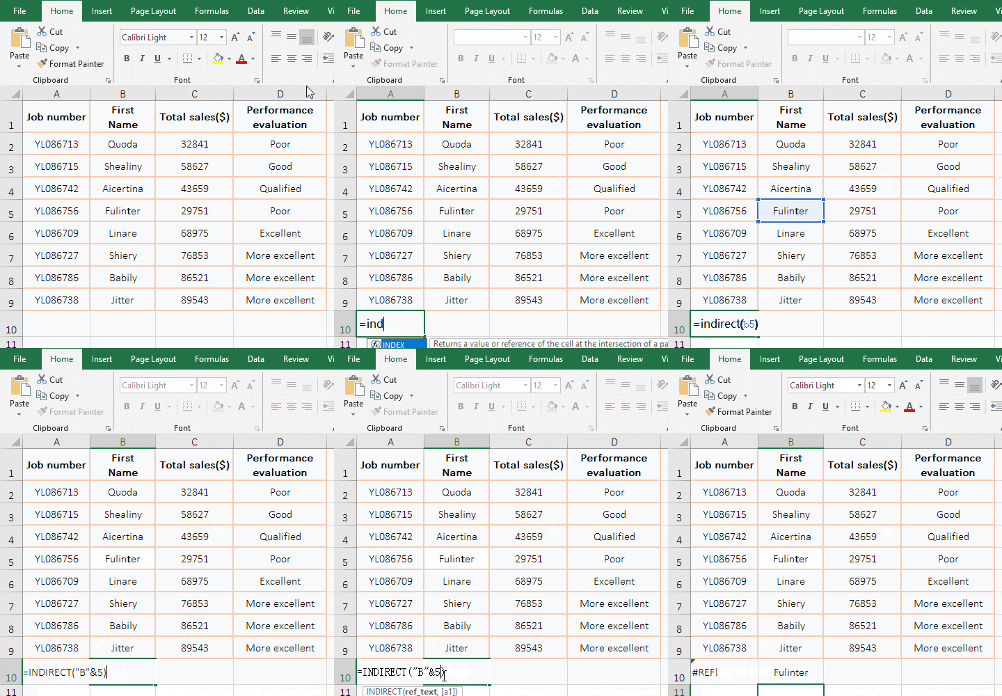
Figure 1

2. Formula description(Excel indirect cell reference):

A. The reason for returning a reference error by the formula =Indirect(B5) is because the first argument of the Indirect function must be text, and B5 is a reference to the cell.

B. "B"&5 is text in the formula =INDIRECT("B"&5), which means that the character B is connected to 5 with &, that is, "B5"; since "B5" is text instead of the reference to B5, so the Indirect function can return the correct value.

C. The formula =INDIRECT("B"&5) and =INDIRECT("B"&5,true) return the same value, indicating that the Indirect function omits the second argument as if it was set to True; in addition, True can also be replaced with 1, the formula =INDIRECT("B"&5,true) can be changed to =INDIRECT("B"&5,1).

(II) Type of reference A1 is False

1. Double-click the cell B9, copy the formula =INDIRECT("R"&5&"C"&2,FALSE) to B9, press Enter, return to the name "Fulinter" in B5; double-click B9, change FALSE to 0, press Enter, also return the same result; the process steps, as shown in Figure 2:

Figure 2

2. Formula description:

"R"&5 means the fifth row in the formula, "C"&2 means the second column, "R"&5&"C"&2 is connected as "R5C2", indicating the reference to the cell at the intersection of the fifth row and the second column; FALSE means the R1C1-style reference, 0 can be substituted for FALSE; the meaning of the formula is: return the reference to the cell at the intersection of the 5th row and the 2nd column, that is, return the "First Name" in B5.

(III) Excel indirect to another sheet: internal references(same table and cross-table reference)

1. The same table reference; the current sheet is "Fruit1", double-click cell A10, copy the formula =INDIRECT("D"&4) to A10, press Enter, and return to the value 3450 in D4. The cross-table reference, if you want to reference the "Fruit2" in "Fruit1"; Double-click B10, copy the formula =INDIRECT("fruit2!D"&4) to B10, press Enter, return to the value 3675 in D4 in "Fruit2"; the operation steps are as shown in Figure 3:

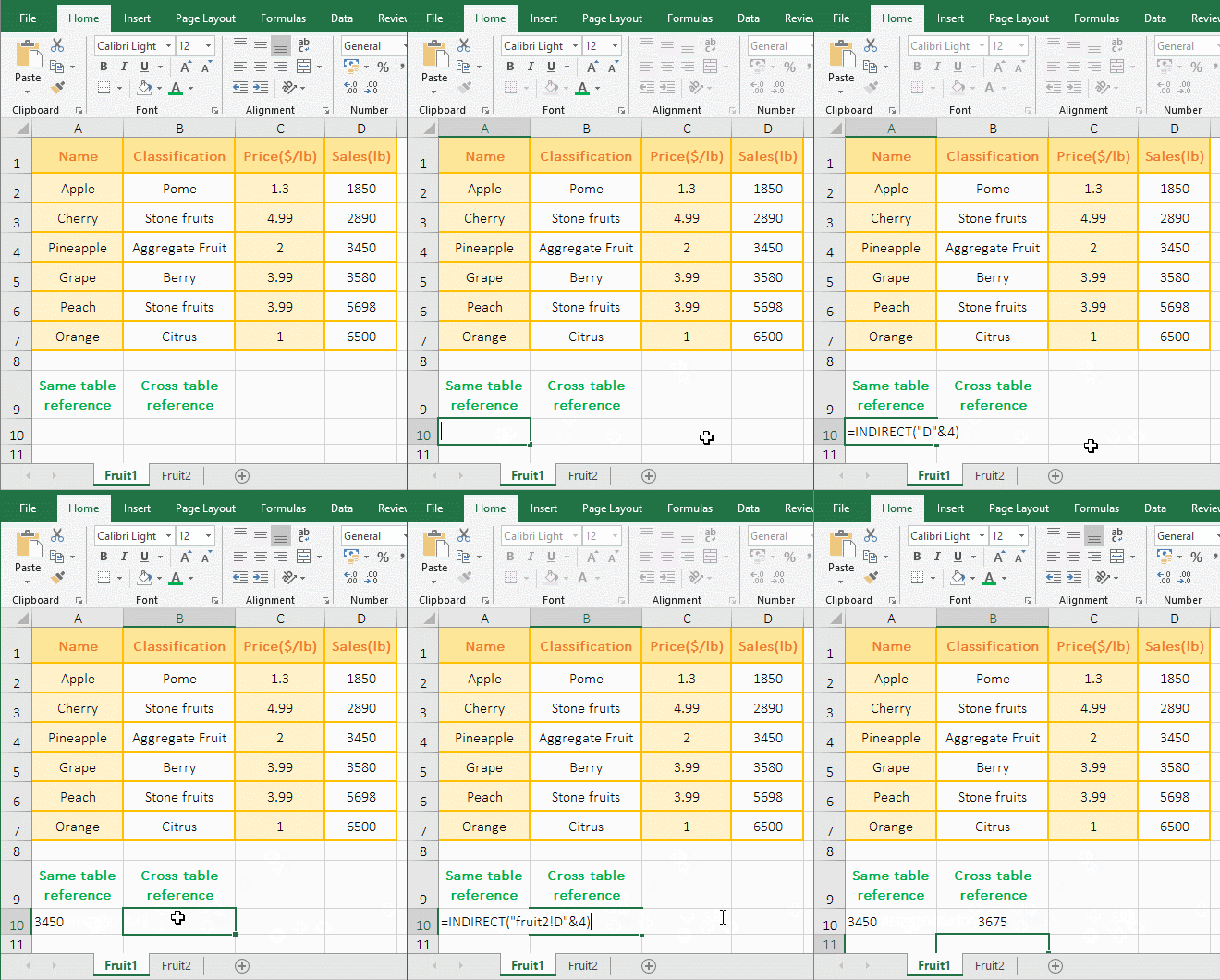
Figure 3

2. Formula description:

The difference between the same table reference and the cross-table reference is: cross-table reference only needs to add the worksheet name and the exclamation mark(ie !) in front of the cell to be referenced. For example, the "fruit2" in the demo is the worksheet name. It is followed by an exclamation mark(!) and D4 is a cell to be referenced.

(IV) Examples of external references(cross-document references)

1. If you want to reference the sales of "White T-Shirt" in the same worksheet in "Clothes2.xlsx" in the "September" worksheet in the document "Clothes1.xlsx". Double-click the cell E6, copy the formula =INDIRECT("[Clothes2.xlsx]September!D6") to E6, press Enter, return to 546; the operation steps are as shown in Figure 4:

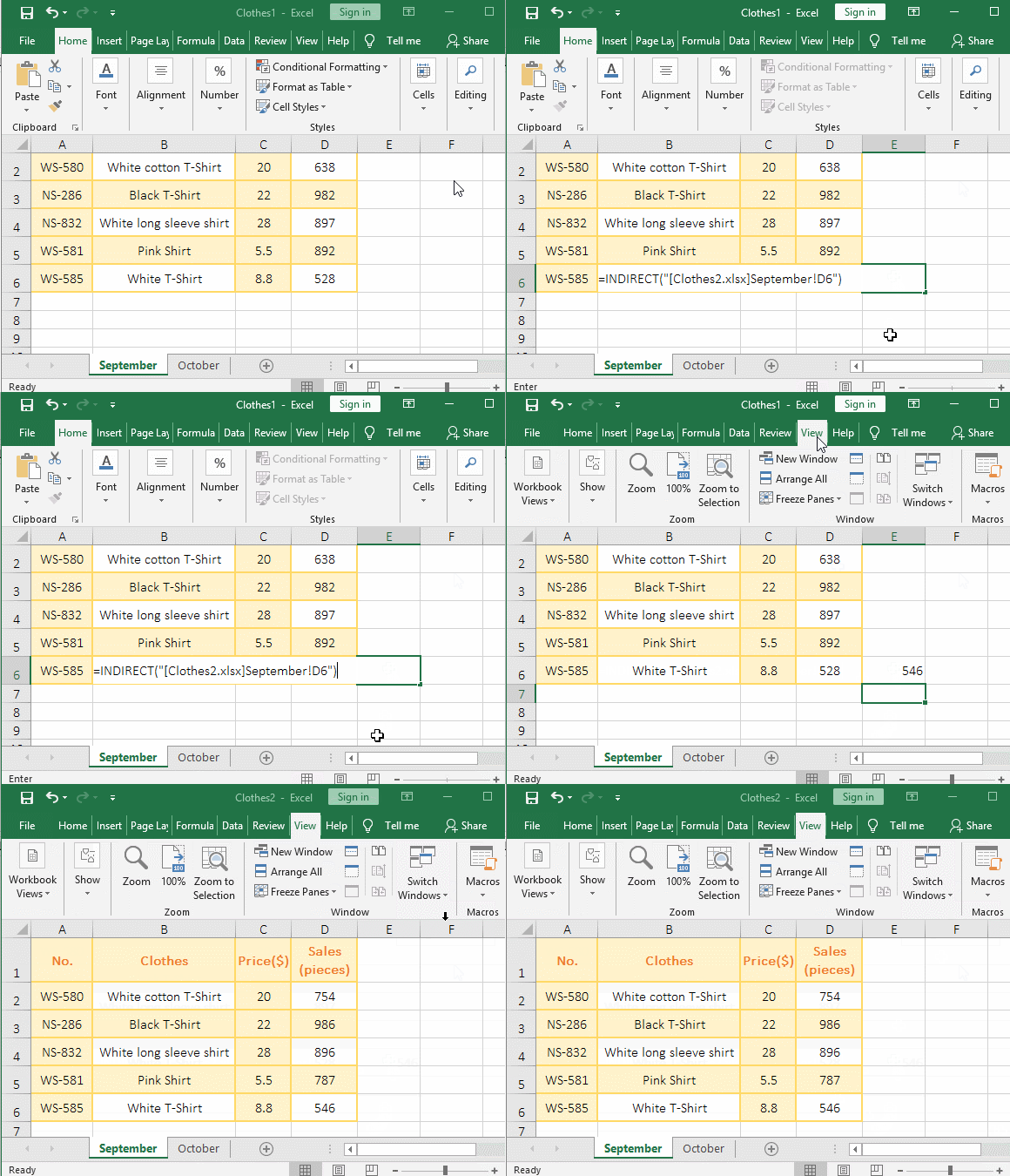
Figure 4

2. Formula description:

[Clothes2.xlsx] is the document name in the formula =INDIRECT("[Clothes2.xlsx]September!D6"), pay attention to the extension ".xlsx"; "September" is the worksheet name, D6 is a cell to be referenced, and an exclamation point(!) is also added between the worksheet name and the cell to be referenced.

(V) The cell to be referenced is the maximum number of rows 1048576 or columns 16384(XFD) allowed by Excel

1. Double-click cell C2, copy the formula =INDIRECT("A"&1048576) to C2, press Enter, return to the maximum number of rows 1048576 allowed by Excel; double-click C2, change the following 6 to 7, press Enter, return the referenced error #REF!; press Ctrl + down arrow to move to the last row, press Ctrl + up arrow to move to the first row. Double-click C3, copy the formula =INDIRECT("XFD"&1) to C3, press Enter, return to the maximum number of columns 16384 allowed in Excel; double-click C2, change XFD to XFE, press Enter, and return the referenced error #REF!; press Ctrl + right arrow to move to the last column, there is no column after the XFD column; press Ctrl + left arrow to move to the first column. Operation process steps, as shown in Figure 5:

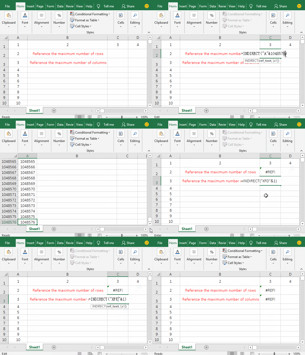
Figure 5

2. Formula description:

When the last row 1048576 is changed to 1048577, the formula returns a referenced error from the demo, indicating that 1048576 is the last row; similarly, the last column XFD is changed to XFE, and the formula also returns a referenced error, indicating that XFD is also the last column.

III, The application examples of Excel Indirect function

(I) Indirect + Row + Address + Column function combination to extract data from a specified row in multiple tables to a table

1. If you want to extract the fourth row of the clothing sales tabel "9, 10 and 11" to the "Sales subtotal". 

The current worksheet is "Sales subtotal", double-click cell A2, copy the formula =INDIRECT(ROW(A9)&"!"&ADDRESS(ROW($A$4),COLUMN(B$1))) to A2, press Enter, return to the clothing name "White long sleeve shirt" in the cell at the intersection of the fourth row and second column in the worksheet 9.

Select A2, move the mouse to the cell fill handle in the lower right corner of A2, after the mouse becomes bold black plus , hold down the left button and drag to the right, drag to C2(The last column of the data table is extracted), then extract the fourth row of the table 9.

Then drag down(The table to extract data is still a few drag a few rows), then extract the data of the fourth row of the worksheet "10 and 11"; switch to the worksheet which data is extracted, you can see that the extracted data is correct; the operation process steps, as shown in Figure 6:

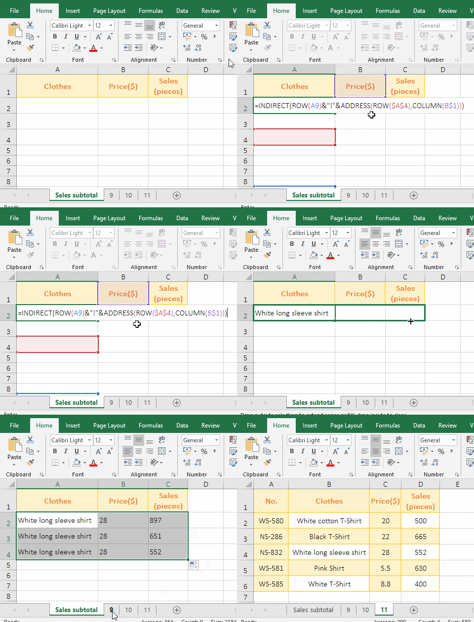
Figure 6

2. Formula =INDIRECT(ROW(A9)&"!"&ADDRESS(ROW($A$4),COLUMN(B$1))) description:

A. ROW(A9) is used to return the row number 9 of A9; when dragging down, A9 will become A10, A11, etc., Row( A10) returns the row number 2, and so on.

B. $A$4 means absolute reference to A4, when dragging down, A4 will not change to A5, A6, etc.; when dragging to the right, A4 will not change to B4, C4, etc.; this ensures that ROW($A$4) always returns to the 4th Row.

C. COLUMN(B$1) is used to return the column number 2 of B1, B$1 is the absolute reference to row and the relative reference to column, to ensure that when dragging to the right, B1 becomes C1, D1, etc., so as to achieve the purpose of taking data of different columns.

D. Then ADDRESS(ROW($A$4),COLUMN(B$1)) becomes ADDRESS(4,2), and then returns the cell at the intersection of the fourth row and second column in text and with absolute reference, ie "$B$4"; because the Address function omits the third argument "type of reference" and is returned with an absolute reference by default.

E. The formula becomes =INDIRECT(9&"!"&"$B$4"), and further calculation, the strings are concatenated, the formula becomes =INDIRECT("9!$B$4"), and finally returns a reference to the B4 in the worksheet 9, that is, returns the clothing name in B4.

(II) Indirect + Match + Column function combination extracts data in batches by criteria
1. If you want to extract earns for any given number of months from a table, the earns per month account for one row. Double-click cell B12, copy the formula =INDIRECT("r"&MATCH($A12,$A$1:$A$9,)&"c"&COLUMN(),0) to B12, press Enter, and return to 74.63; select B12, return the remaining data of "January" with the method of dragging to the right, and then extract the earns of "April, May and August" with the method of dragging downward to; the operation process steps, as shown in Figure 7:

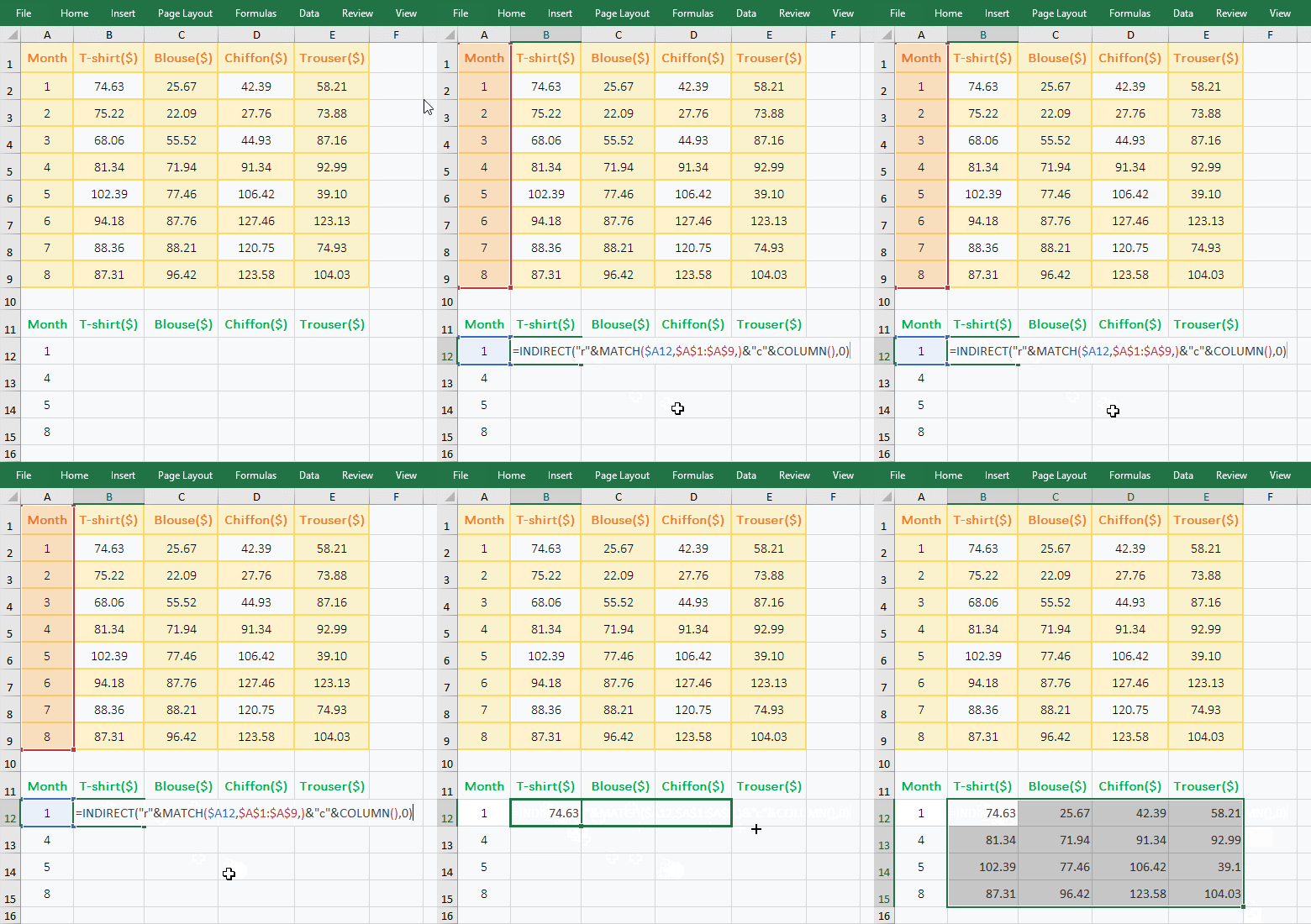
Figure 7

2. Formula =INDIRECT("r"&MATCH($A12,$A$1:$A$9,)&"c"&COLUMN(),0) explanation:

A. MATCH($A12,$A$1:$A$9,) is used to return the position of A12(ie "January") in A1:A9, the result is 2; $A12 is the absolute reference to column and relative reference to row, it is changed to B12 when dragging to the right, and is changed to A13 when dragging downwards, so as to get "April in A13, May in A14", etc.; the columns and rows of $A$1:$A$9 are absolutely referenced because always make sure to lookup in A1:A9 when dragging down, because with absolute reference, dragging down, A1 will not be A2, A9 will not change to A10. In addition, the Match function omits the first argument, and the default is 0, indicating an exact match.

B. COLUMN() is used to return the column number of the cell in which the formula is located, when the formula is B12, it returns 2; when the formula has C12, it returns 3, and so on.

C. The formula becomes =INDIRECT("r"&2&"c"&2,0), further calculations, connect the characters, and the formula becomes =INDIRECT("r2c2",0). r represents the row number. c is the column number, 0 is in the r1c1-style reference in the formula, and the formula returns the reference to the cell at the intersection of second row and second column, which returns the value 74.63 in B2.