 Office > Excel > Excel 2019 > Content
How to calculate standard deviation in excel(6 function, with Stdev,Stdev.S,StdevA,StdevP)
The standard difference is the standard deviation of sample and the standard deviation of population. The former refers to extracting some data from a population as sample to calculate the standard deviation, and the latter refers to calculating the standard deviation for all data, and it is often impossible to obtain all the data in reality. Therefore, it generally calculats the standard deviation of the sample. There are 6 functions for Excel standard deviation calculation, but there are actually only 4, because there are two new ones that are only used to replace the old functions, they are the same as the old ones. Stdev, Stdev.S, and StdevA are used to calculate the standard deviation of the sample. StdevP, Stdev.P, and StdevPA are used to calculate the standard deviation of the entire population.
In addition to calculating the standard deviation of a set of values, it is also possible to calculate the standard deviation that meets two or more conditions. In addition, the standard deviation function can be combined with the OffSet and Match functions to automatically calculate the standard deviation and calculate the standard deviation of the last few days after adding data.
I, The calculation function of standard deviation in Excel
(I) Calculation function of standard deviation of sample
1. Expression
Stdev function expression: STDEV(Number1,[Number2],...)
Stdev.S function expression: STDEV.S(Number1,[Number2],...)
StdevA function expression: STDEVA(Value1,[Value2],...)
2. Description:
A. Stdev function and Stdev.S function are used to calculate the standard deviation of sample, they must use one argument at least, up to 255; Stdev.S function is added in Excel 2010, used to replace the Stdev function, In future versions of Excel, the Stdev function may not be supported anymore.
B. The StdevA function can calculate the standard deviation of sample of the logic(True or False) and text values in addition to calculate the standard deviation of sample of the value; it must also have at least one Value and a maximum of 255 Values.
C. Stdevn(Stdev.S) and StdevA function difference: their difference is limited to how to deal with logical values and text values, for logical values and text values, if input directly into the list of argument, they are included in the calculation of standard deviation by Stdev function, True is converted to 1, False is converted to 0; if they are in an array or cells to be referenced, the Stdev function ignores them. The StdevA function counts the logical and text values into the standard deviation, regardless of where they are entered. In addition, if there are texts in the argument list that cannot be converted to numeric values, they all return an error; if there are texts that cannot be converted to a numeric value in the array or cells to be referenced, they are ignored.
(II) Calculation function of the standard deviation of population
1. Expression
StdevP function expression: STDEVP(Number1,[Number2],...)
Stdev.P function expression: STDEV.P(Number1,[Number2],...)
StdevPA function expression: STDEVPA(Value1,[Value2],...)
2. Description:
A. StdevP function and Stdev.P function are also used to calculate the standard deviation of population of the values, they must use one argument at least, up to 255; Stdev.P function is also added in Excel 2010, used to replace StdevP function, StdevP function may be abandoned in a future version of Excel.
B. The StdevPA function is used to calculate the standard deviation of population of the logical(True or False) and text values in addition to be used to calculate the standard deviation of population of the values; it must also have at least one Value and a maximum of 255 values.
C. StdevP function(Stdev.P function) and StdevPA function difference: their difference is also limited to how to deal with logical values and text values, for logical values and text values, if they are inputted directly into the argument list, they are included in the calculation of the standard deviation by StdevP function, True is converted to 1, False is converted to 0; if they are in an array or cells to be referenced, the StdevP function ignores them. The StdevPA function counts the logical and text values into the calculation of the standard deviation. In addition, if there are texts that cannot be converted to numeric values in the argument list, they all return an error; if there are texts that cannot be converted to the numeric value in the array or cells to be referenced, they are also ignored.
II, How to calculate standard deviation in excel(standard deviation of sample)
(I) Calculate the standard deviation of the values with Stdev(Stdev.S)
(1) Examples of calculations with Stdev and Stdev.S
1. If you want to calculate the standard deviation of sample of English scores. Double-click cell B2, copy the formula =STDEV(B2:B18) to B2, press Enter, return to 8.389857322; double-click B3, copy the formula =STDEV.S(B2:B18) to B3, press Enter, and return to 8.389857322; select B2:B3, the current tab is "Home", click the black small inverted triangle to the right of "General", select "Number" in the pop-up options, the standard deviation are round up to two decimals; the operation steps, such as Figure 1 shows:
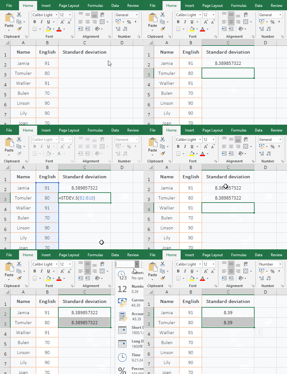
Figure 1
2. Formula description:
A. B2:B18 is the cells to be referenced for calculating the standard deviation, the results returned by the two formulas are the same, indicating that Stdev works the same as Stdev.S.
B. The result returned by the formula rounds up to multiple decimal places by default, only two decimal places are rounded up to in the demo. If you want to round up to other decimal places, you can press Ctrl + 1 to open the "Format Cells" Window, select the "Number" tab, then select the "Number" on the left, then enter the specific value in the "Decimal Places" on the right, click "OK".
(2) True and False are counted and ignored
1. True and False are included in the calculation of standard deviation
A. Double-click cell A1, copy the formula =STDEV(24,27) to A1, press Enter, return to 2.121320344; double-click A2, copy the formula =STDEV(24,27,TRUE) to A2, press Enter, return 14.2243922; double-click A3, copy the formula =STDEV(24,27,FALSE) to A3, press Enter, return to 14.79864859; the operation steps are as shown in Figure 2:
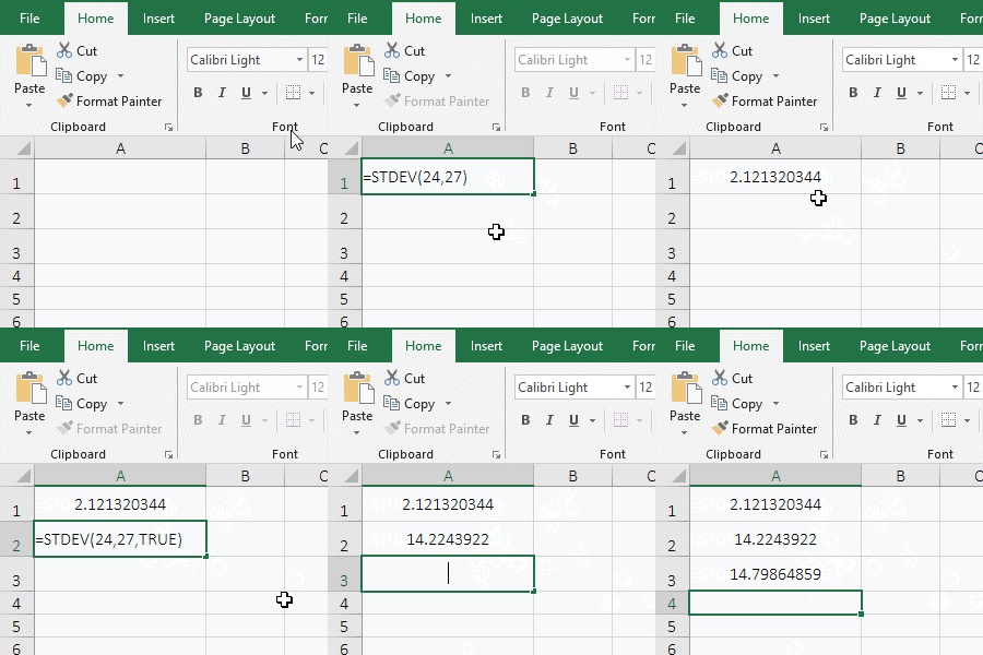
Figure 2
B. Formula description:
The formula =STDEV(24,27,TRUE) and =STDEV(24,27,FALSE) return different results than =STDEV(24,27), indicating that both TRUE and FALSE are counted in the calculated standard deviation, which shows that the logical value is written directly to the argument list of the Stdev function and is included in the standard deviation.
2. True and False are ignored when calculating the standard deviation
A. Double-click cell C2, copy the formula =STDEV(A2:A3) to C2, press Enter, return to 2.121320344; double-click C3, copy the same formula to C3, then change the formula to =STDEV(A2:A4), press Enter, also returns 2.121320344; select B4, change TRUE to false, click C3, the value in C3 has not changed; double-click C6, copy formula =STDEV({24,27,TRUE,FALSE}) to C2, press Enter, also returns 2.121320344; the operation process steps, as shown in Figure 3:
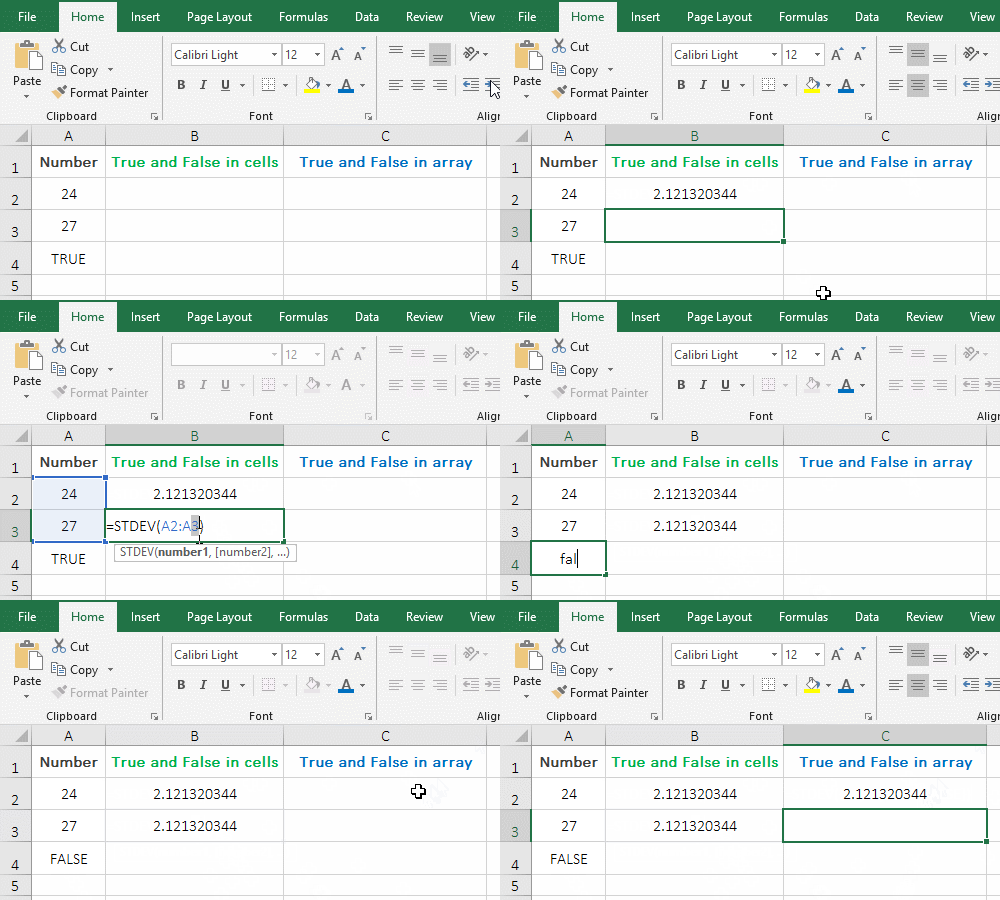
Figure 3
��B. Formula description:
As you can see from the demo, each formula returns the same result regardless of whether it contains True or False, indicating that True and False are ignored in the cells or array by Stdev function.
(3) There are texts that can be converted to values are counted and ignored.
1. Double-click cell A1, copy the formula =STDEV(2.58,2.39,"2.67") to A1, press Enter, return to 0.142945211; double-click A1 again, delete ", 2.67", press Enter, return to 0.134350288; double-click A2, copy the formula =STDEV(B1:B3) to A2, press Enter, return to 0.134350288; the operation steps are as shown in Figure 4:
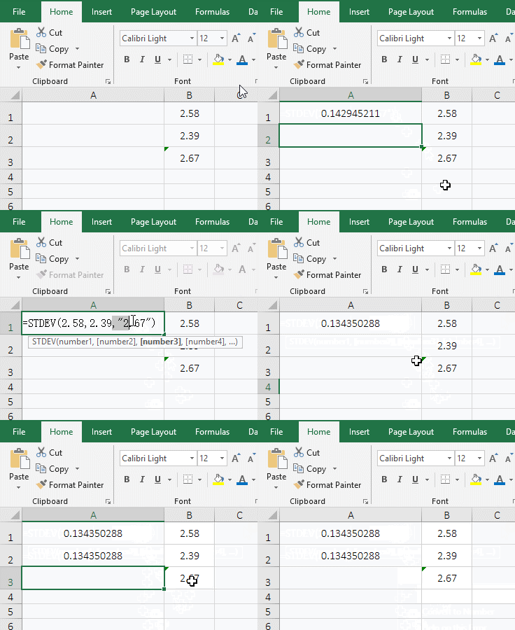
Figure 4
2. Formula description:
The result returnd by the formula =STDEV(2.58,2.39,"2.67") is not the same as the result returned by =STDEV(2.58,2.39), indicating that the numeric text "2.67" is included in the calculation of standard deviation; and the result returned by the formula =STDEV(B1:B3) and =STDEV(2.58, 2.39) is the same, indicating that 2.67 in B3 does not be counted in the calculated standard deviation because it is text.
(4) Return errors because there are texts that cannot be converted to numeric values and are ignored
1. Double-click cell A1, copy the formula =STDEV(2.58,2.39,"Ten") to A1, press Enter, return the value error #VALUE!; double-click A2, copy the formula =STDEV(B1:B3) to A2, press Enter, return to 0.134350288; the operation steps are as shown in Figure 5:
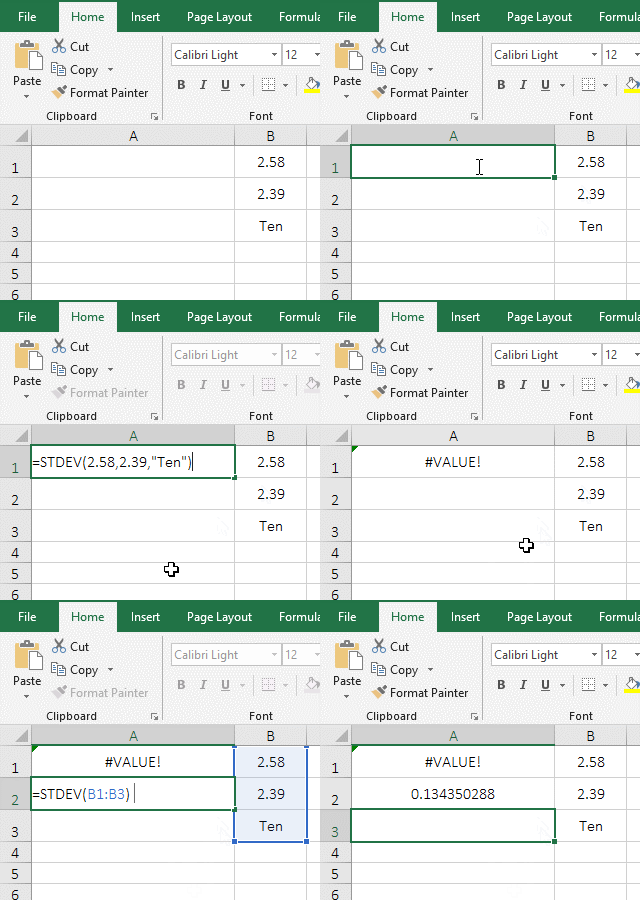
Figure 5
2. Formula description:
The two formulas calculate the standard deviation of the same value and text. The formula =STDEV(2.58,2.39,"Ten") returns an error indicating that text that cannot be converted to a value cannot be written to the argument list; instead, formula =STDEV(B1:B3) can return the correct value, indicating that the array or cells to be referenced have text that cannot be converted to a value, and the text is ignored without affecting the calculation.
(II) Calculate the standard deviation of numerical values, text values, and logical values with StdevA
(1) There are numeric values, text values, and logical values in the cells to be referenced
1. Double-click cell B2, copy the formula=STDEVA(A2:A6) to B2, press Enter to return to 47.00850987; select A4, delete 86, the value in B2 becomes 49.47305664, select A5, delete True, the value in B2 is changed to 49.81298358, and delete the False in A6, and the value in B2 is changed to 5.658854249; the operation steps are as shown in Figure 6:
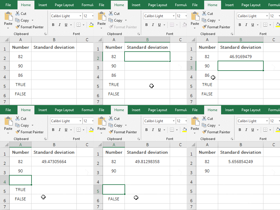
Figure 6
2. Formula description:
The values in A2 and A3 are numeric, and the values in A4 are text. When the value in A4 is deleted, the result of standard deviation is changed from 47.00850987 to 49.47305664, indicating that the StdevA function counts the text in the cell into the calculated standard deviation. When the True and False are deleted in turn, the result of standard deviation also changes, indicating that the StdevA function counts the logical value into the standard deviation.
(2) StdevA and Stdev compare and count examples of text numeric counts and ignores
1. Whether the text values are written directly to the argument list or written to the cells, they are included in the standard deviation by StdevA, but the processing of the decimal is not the same. For example, the results of calculation in E3, E4, and E5 are different, indicating that StdevA counts the text value into the standard deviation; when writing directly "2.67" to the argument list, the text type "2.67" is converted to the numeric 2.67, and When 2.67 in cell is the text, it is replaced by the decimal point and then converted to a number. The result after conversion to a value is 267. This can be confirmed by changing 2.67 in C5 to 267 and the result in E5 dose not change. The demo is shown in Figure 7:
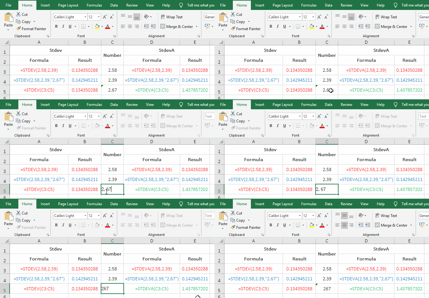
Figure 7
2. The difference between StdevA and Stdev for text values is: Stdev only counts the text value "2.67" written directly into the argument list in the standard value, and StdevA counts the text value "2.67" in the argument list and cells in the standard deviation. In Fig. 7, the calculation results of the same color are the same, that is, the text values are processed in the same manner.
III, How to calculate standard deviation in excel(standard deviation of population)
(I) An example of calculating the standard deviation of population with StdevP and Stdev.P
1. Double-click cell B2, copy the formula =STDEVP(A2:A6) to B2, press Enter, return to 0.681791757; double-click B3, copy the same formula to B3, and then add a point before P, the formula becomes =STDEV.P(A2:A6), press Enter to return the same result; the operation steps are as shown in Figure 8:
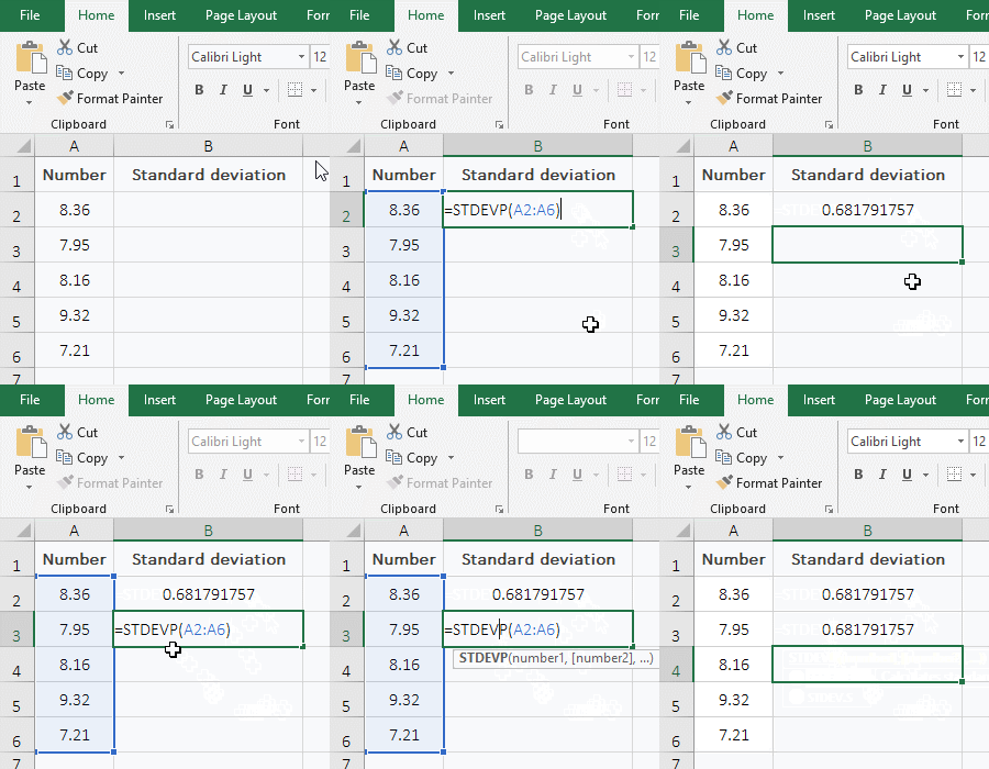
Figure 8
2. Formula description:
The formula =STDEVP(A2:A6) and =STDEV.P(A2:A6) return the same result, indicating that they all work together to calculate the standard deviation of population of the values.
(II) Calculate the standard deviation of population containing numerical values, text values, and logical values with StdevPA
1. Double-click cell B2, copy the formula =STDEVPA(A2:A6) to B2, press Enter, return to 3.851360279; select A4, delete the text value 8.16, the value in B2 becomes 3.846526842; delete False in A5 , the value in B2 becomes 3.377490995; then delete the True in A6 , the value in B2 becomes 0.205; the operation steps are as shown in Figure 9:
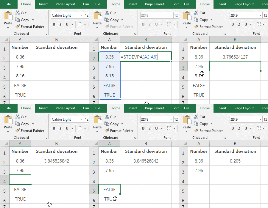
Figure 9
2. Formula description:
When the text value in A4 is deleted, the result of standard deviation changes, indicating that the StdevPA function counts the text value into the standard deviation; then deletes True and False, and the result of standard deviation also changes, indicating that the StdevPA function also counts the logical value into the standard deviation.
Hint: The difference between the StdevP and StdevPA function for the processing of numeric text, logical values, and text that cannot be converted to values, please refer to the difference between the Stdev and StdevA function.
IV, The application examples of calculation function of standard difference in Excel
(I) Calculating the standard deviation of the sample that meets two criteria
1. If you want to calculate the standard deviation of sample of the sales of "Sweater" in New York. Double-click cell D12, copy the formula =STDEV((B2:B11="Sweater")*(C2:C11="New York")*(D2:D11)) to D12, press Ctrl + Shift + Enter to return the result 728.2405; operation process steps, as shown in Figure 10:
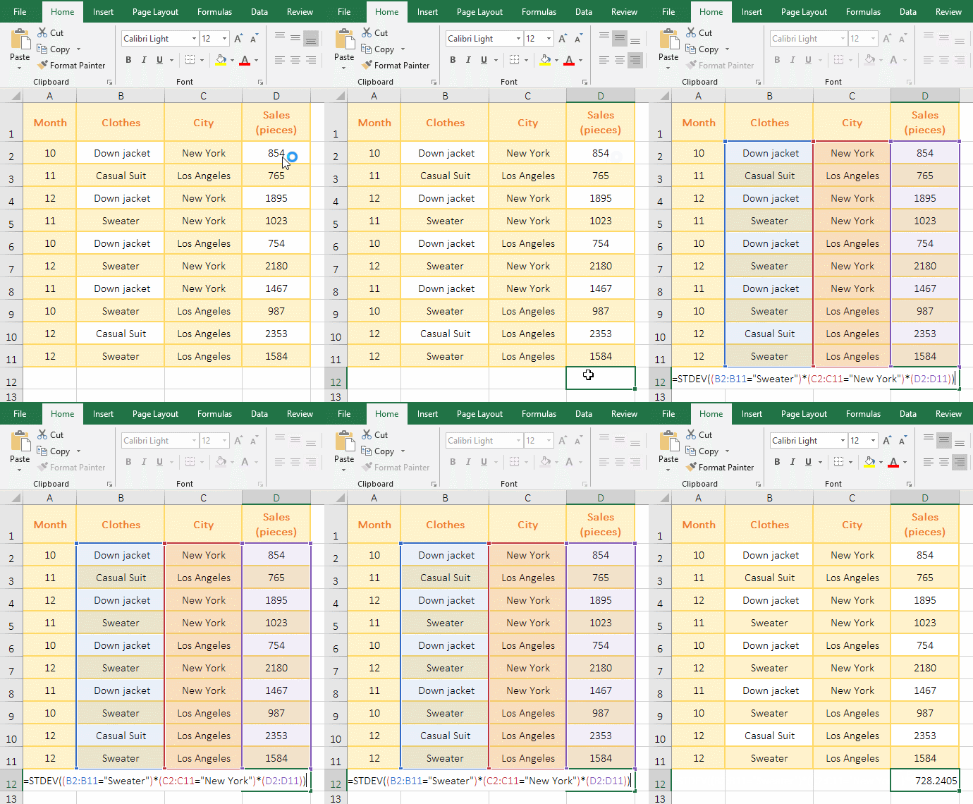
Figure 10
2. Formula =STDEV((B2:B11="Sweater")*(C2:C11="New York")*(D2:D11)) description:
A. B2:B11="Sweater" is the first criteria of the formula, meaning: lookup the "Sweater" in B2:B11, if it is "Sweater", return True, otherwise return False. At the time of execution, B2 is taken out from B2:B11 for the first time; since B2 is "Down jacket", it returns to False; B3 is taken out from B2:B11 for the second time, and since B3 is "Casual Suit", it also returns to False; other and so on, and finally return the array {FALSE;FALSE;FALSE;TRUE;FALSE;TRUE;FALSE;TRUE;FALSE;TRUE}.
B. C2:C11="New York" is the second criteria of the formula, meaning: lookup the "New York" in C2:C11. If it is "New York", it returns True, otherwise it returns False, and finally returns Array {TRUE;FALSE;TRUE;TRUE;FALSE;TRUE;TRUE;FALSE;FALSE;FALSE}.
C. Then (B2:B11="Sweater")*(C2:C11="New York") becomes {FALSE;FALSE;FALSE;TRUE;FALSE;TRUE;FALSE;TRUE;FALSE;TRUE}*{TRUE;FALSE ;TRUE;TRUE;FALSE;TRUE;TRUE;FALSE;FALSE;FALSE}, then, first, the first element of the first array is multiplied by the first element of the second array, and the result is 0(because True is Converted to 1, False is converted to 0); second, takes the second element of the first array and multiplies the second element of the second array, the result is 0; the other and so on, and finally returns the array {0;0;0;1;0;1;0;0;0;0}.
D. D2:D11 returns the values in D2 to D11 as an array, which returns {854;765;1895;1023;754;2180;1467;987;2353;1584}.
E. Then the formula becomes =STDEV({0;0;0;1;0;1;0;0;0;0}*{763;692;1090;969;583;1286;990;686;960; 986}), then, multiplying the corresponding elements of the two arrays, the formula is further changed to =STDEV({0;0;0;969;0;1286;0;0;0;0}), and finally the standard deviation of sample is obtained by Stdev.
Hint: The above is to calculate the standard deviation of sample that meets two criteria. If you want to calculate the standard deviation of sample that meets three or more criteria, you can continue to add criteria after the second * of the formula. Also, if you want to calculate the standard deviation of population, change Stdev to StdevP.
(II) Stdev + OffSet + Match combination to automatically calculate the standard deviation after adding new data and calculate the standard deviation of the last few days
(1) Calculate the standard deviation of sample of all data
1. If it is required to automatically calculate the standard deviation of sample of the index for each additional "Index". Double-click the cell C3, copy the formula =STDEV(OFFSET(B1,1,,MATCH(9E+307,B:B)-1)) to C3, press Enter, return the result 71.0624; select A8, enter "7", press the Tab key to move the cursor to B8, enter 837, click A9, the value in C3 will automatically change to 64.9300, which means that the standard deviation containing the newly added data is recalculated automatically after adding a row; continue to input data in A9 and B9, press Enter, the value in C3 will automatically change to 68.3013; the operation steps are as shown in Figure 11:
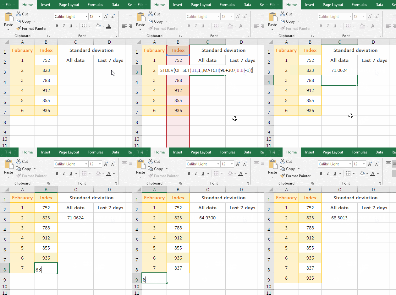
Figure 11
2. Formula =STDEV(OFFSET(B1,1,,MATCH(9E+307,B:B)-1)) description:
A. 9E+307 is the maximum value allowed by Excel, which is used to represent the last row. MATCH(9E+307,B:B) is used to return the position of the last row in column B; when the table has only 7 rows, it returns 7; Match omits the last argument, which defaults to 1, because there is no comma after the second argument B:B, which means: Lookup the maximum value that is less than and equal to 9E+307 in column B and return it the position in column B.
B. Then OFFSET(B1,1,,MATCH(9E+307,B:B)-1) becomes OFFSET(B1,1,,7-1), then, based on B1, returns the reference to the cell at the intersection of 1 row under B1 and 0 column to right of B1 and height to 6 and width to 1, that is, returns $B$2:$B$7. The OffSet function omits the third argument column number, the default value is 0. The fifth argument width is also omitted, the width is the same as B1 by default, that is, 1 is taken.
C. The formula becomes =STDEV($B$2:$B$7), and finally the standard deviation of sample is calculated for all the values in B2:B7.
D. When adding a row after the table, MATCH(9E+307,B:B) returns 8, and OFFSET(B1,1,,8-1) returns $B$2:$B$8, which just contains the newly added row. Therefore, new data is automatically counted into the standard deviation after adding new data.
(2) Calculate the standard deviation of sample of the last 7 days
1. Double-click cell D3, copy the formula =STDEV(OFFSET(B1,MATCH(9E+307,B:B)-1,,-7)) to D3, press Enter, return the result 58.5800; operation procedure, as shown in Figure 12:
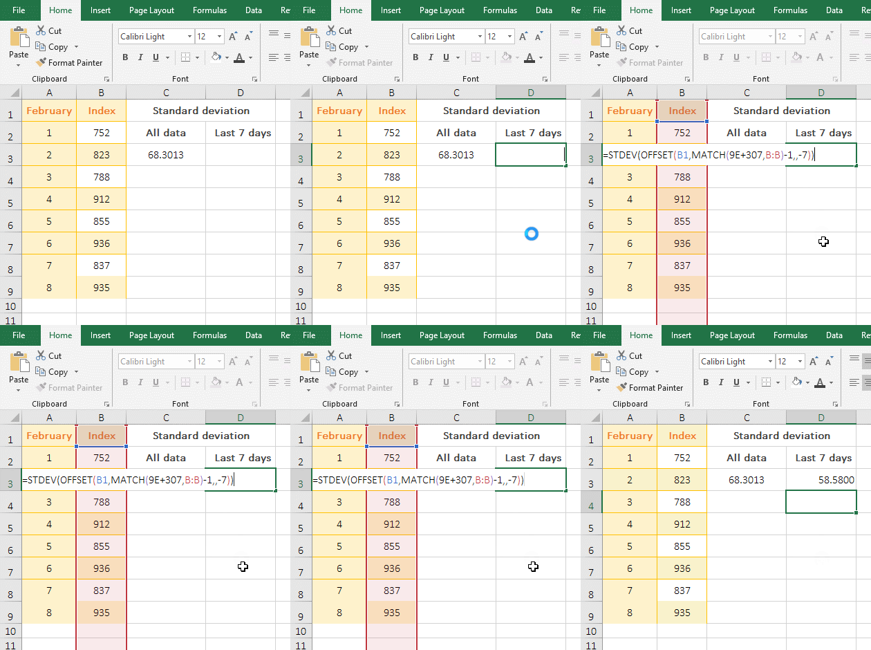
Figure12
2. Formula =STDEV(OFFSET(B1,MATCH(9E+307,B:B)-1,,-7)) description:
A. MATCH (9E+307,B:B) is also used to return the position of the last row in column B in the table, and the result is 9.
B. Then OFFSET(B1,MATCH(9E+307,B:B)-1,,-7) becomes OFFSET(B1,9-1,,-7), and then, based on B1, returns the reference to the cell at the intersection of 8 row under B1 and 0 column to right of B1 and height to -7 and width to 1, that is, returns $B$3:$B$9. The next 8 rows of B1 are up to B9, and -7 means from bottom to top, here, it means: from B9 to the top 7 rows, that is, B3.
C. The formula becomes =STDEV($B$3:$B$9), and finally the standard deviation of sample is calculated for the values in B3:B9, that is, the standard deviation of the last 7 days is calculated. If you want to calculate 5 or 14 days, change -7 to -5 or -14.
-
Related Reading
- How to move rows,columns,cells,table in excel(there
- Excel CountA and CountBlank function usage examples(
- 8 examples of Excel Match function, include it and S
- How to use offset function in excel, include it and
- Excel SumProduct function(multiple criteria, with if
- How to use Excel small function and it and index, ma
- Excel left function usage(8 examples, with Sum+Value
- How to use Average function in excel(combine with if
- How to adjust row height and change width of column
- Excel If function examples, include if statement nes
- How to use Excel address function(7 examples, with I
- Excel SumIf function with ?/*, Average and array mul