 Office > Excel > Excel 2019 > Content
How to create Excel dynamic chart with option button or combo box-show turnover each month and store
You need to use a combo box or option button control to make a dynamic chart in Excel. If only one item of data is displayed dynamically, you can use a combo box; if you want to display more than two items of data, you need to use an option button and a combo box to combine. For example, to dynamically display the Production and Quantity Passed of products produced each month, you can complete it with a combo box; and to dynamically display the turnover of each month or each store, you need to use option buttons and combo boxes.
How to create dynamic charts in excel? You make a dynamic chart in Excel needs to use the OffSet function, return a reference to the corresponding cell according to the currently selected value by it. If you only use a combo box, you don't need to define a name. If you use an option button to combine with a combo box, you need to define a name.
I, Excel displays "Developer" tab
Excel does not display the "Developer" tab by default, you need to display it first, the method: right-click on any blank space in the ribbon, select"Customize the Ribbon" in the pop-up menu, open the "Excel Options" dialog box, and automatically select "Customize Ribbon", check "Developer" under "Main Tab", and click "OK", then the "Developer" will be displayed on the ribbon; the operation steps are shown in Figure 1:
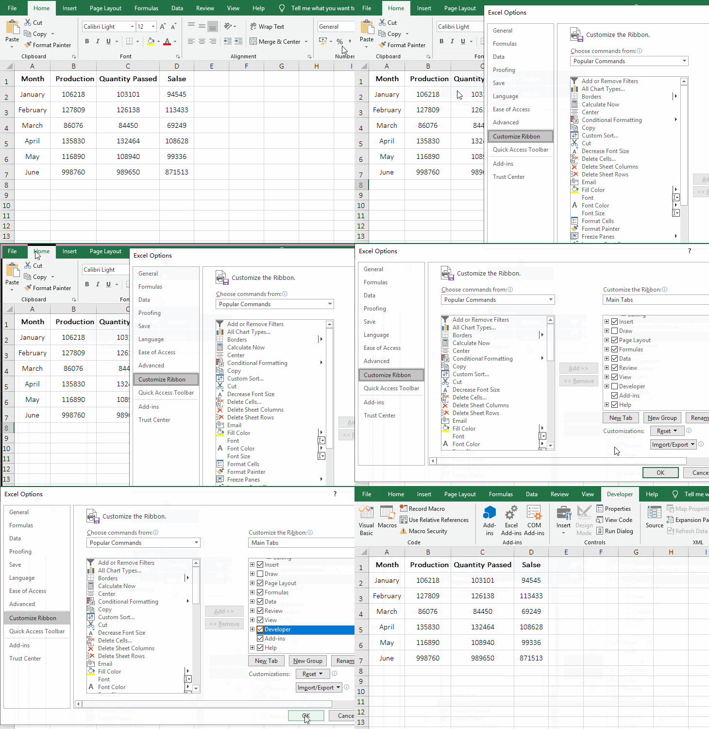
Figure 1
II, How to create Excel dynamic chart
1. How to insert a combo box in excel
A. Select the "Developer" tab, click "Insert", select "Combo Box" under "Form Control", the mouse is changed to the "plus", move it to the position where you want to draw the combo box, hold down the left button and drag, draw a combo box with the right size and release the left button, a combo box is successfully inserted;
B. Right-click the combo box, select "Format Control" from the pop-up menu to open the "Format Control" dialog box, position the cursor to the right of "Input range", and select A2:A7 as the "Input range" of the combo box(if the "Input range" has a lot of rows. You can enter it directly. Note that $ is added to indicate absolute reference.). Then position the cursor to the left of "Cell link" and select a cell(such as J3) as the index(serial number) of the current selection value of the combo box, click "OK" to add "Month" as the "Input range" of the combo box;
C. Click any blank space to release the selected state of the combo box, and then click it to expand the "Months" that were just added, select "February", 2 is displayed in J3, and then select "April", J3 display 4; the oeration process steps, see screenshot in Figure 2:
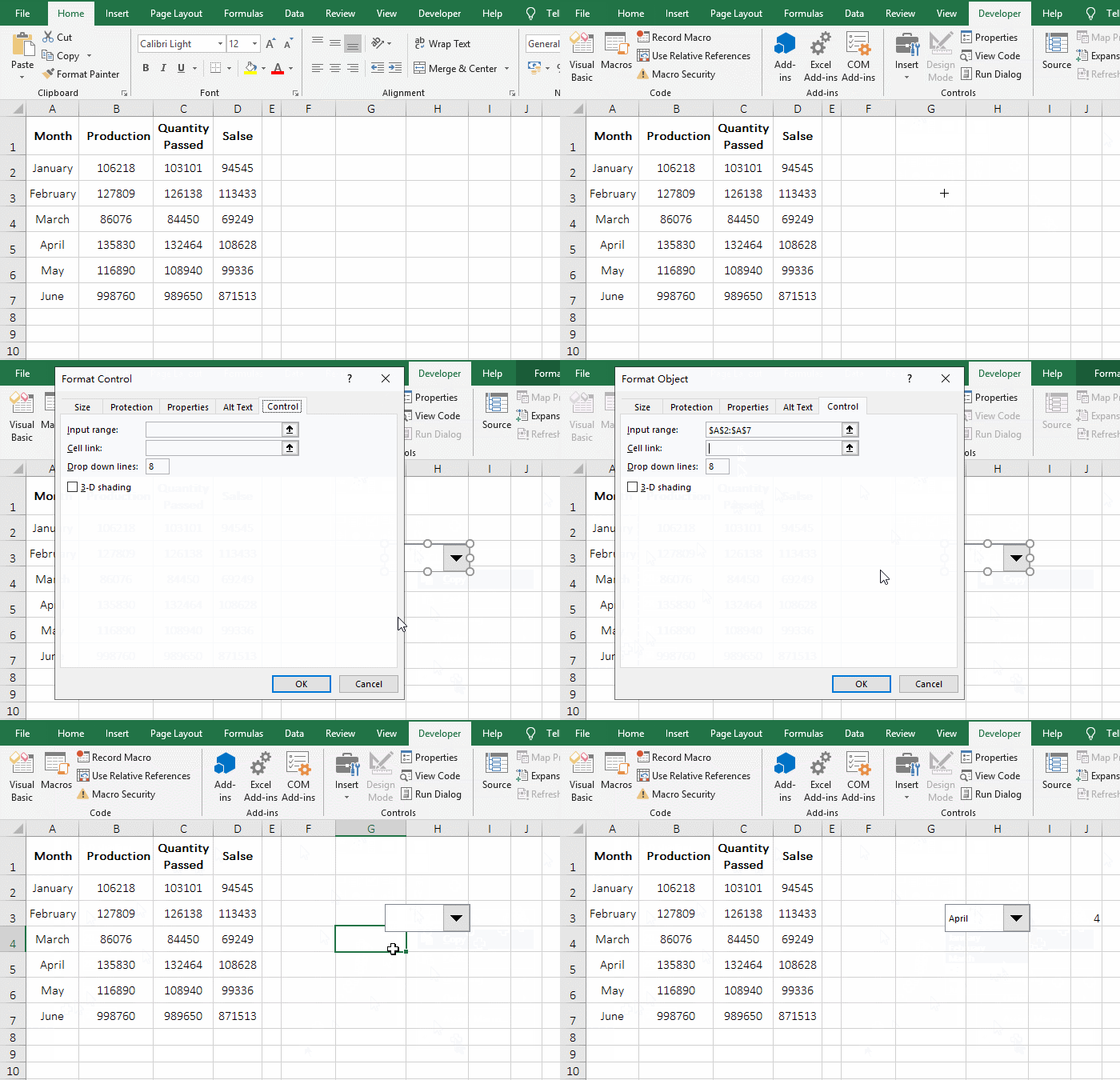
Figure 2
2. Copy the header and display the corresponding record according to the selection value of the combo box(ie Excel chart dynamic range)
A. Select A1:D1, select the header, press Ctrl + C to copy, select F1, press Ctrl + V, and paste a copy of the header;
B. Select F2, select the "Formulas" tab, click "Lookup & Reference", select OFFSET from the pop-up options, open the "Function Arguments" dialog box, click A1, then A1 is automatically entered into the input box of the "Reference"; enter J3 into the input box to the right of the "Rows" in the same way, and then change the references of the two input boxes to $A$1 and $J$3; position the cursor to the input box to the right of the "Cols", copy COLUMN(A1)-1 into it, click "OK", then the value in F2 becomes "April", which is the value of the combo box;
C. Select F2 and move the mouse to the cell fill handle in the bottom right of F2, after the mouse changes to a bold black plus sign, hold down the left button and drag right until to I2, and the data of "April" is extracted; click the combo box, select "January", the data in F2:I2 are automatically changed the data of "January". The operation steps are shown in Figure 3:

Figure 3
D. Formula =OFFSET($A$1,$J$3,COLUMN(A1)-1) explanation:
(1) What is set in the "Function Arguments" dialog box is actually the formula =OFFSET($A$1,$J$3,COLUMN(A1)-1). The meaning of the formula is: based on A1, return the reference to cell rows 4 under A1(The value in J3 is 4) and column 0(The value of COLUMN (A1) -1) value is 0), which returns a reference to A5, which is "April".
(2) $A$1 means absolute references to both row and columns. When dragged down, A1 will not change to A2, A3, etc .; when dragged to the right, A1 will not change to B1, C1, etc.; $J$3 is the same as the $A$1.
(3) COLUMN(A1) returns the column number 1 of A1, and COLUMN(A1)-1 is equal to 0; when the formula is dragged to G2, COLUMN(A1)-1 becomes COLUMN(B1)-1, and the result is 1; then OFFSET($A$1,$J$3,COLUMN(A1)-1) becomes OFFSET($A$1,1,1), which returns a reference to cell row 1 under A1 and column 1 to the right of A1, which returns a reference to B2.
Hint: If you are not familiar with the OffSet function, check out the article "How to use offset function in excel, include it and Sum, Match, CountIf combination in formula".
3. Generate dynamic charts.
A. Select the "Insert" tab, click the "Insert Column or Bar Chart" icon, and select the first "Clustered Column" in the pop-up chart style to insert a chart. Move the mouse to the chart, after the mouse becomes a cross with four arrows, press and hold the left button to move the chart to the right position.
B. Right click the chart, select "Send to Back → Send to Back" in the pop-up menu, move the chart to the bottom, and prevent it from blocking the combo box. If there are not many things inserted in the document, you can also move down layer by layer. Right-click the combo box to select it, and hold down the left mouse button to move the combo box to the top right of chart.
C. Right click the chart, select "Select Data" from the pop-up menu, open the "Select Data Source" dialog box, select F1:I2, change the "Chart data range" to the selected range, and click "OK", then the X axis becomes "Month" in the chart, click "Combine box" and select "March", then the chart will display the data of "March", and then select "May", then the chart will display the data of "May"; operation steps , see screenshot in Figure 4:
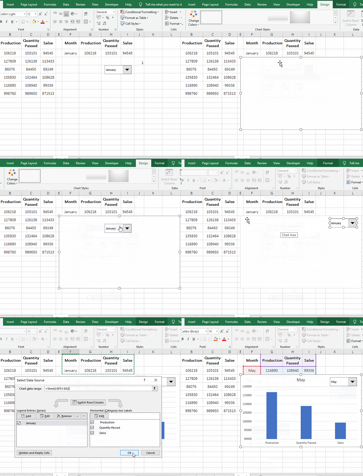
Figure 4
III, How to make Excel dynamic chart with the double combo box control
1. Copy the table header. Select cell B1, hold down Shift, click G1, select B1:G1, the current tab is "Home", select A9, click "Paste" in the top right of the screen, and select "Transpose" under "Paste" from the pop-up options, the column header of table are converted to rows; the operation process steps are shown in Figure 5:
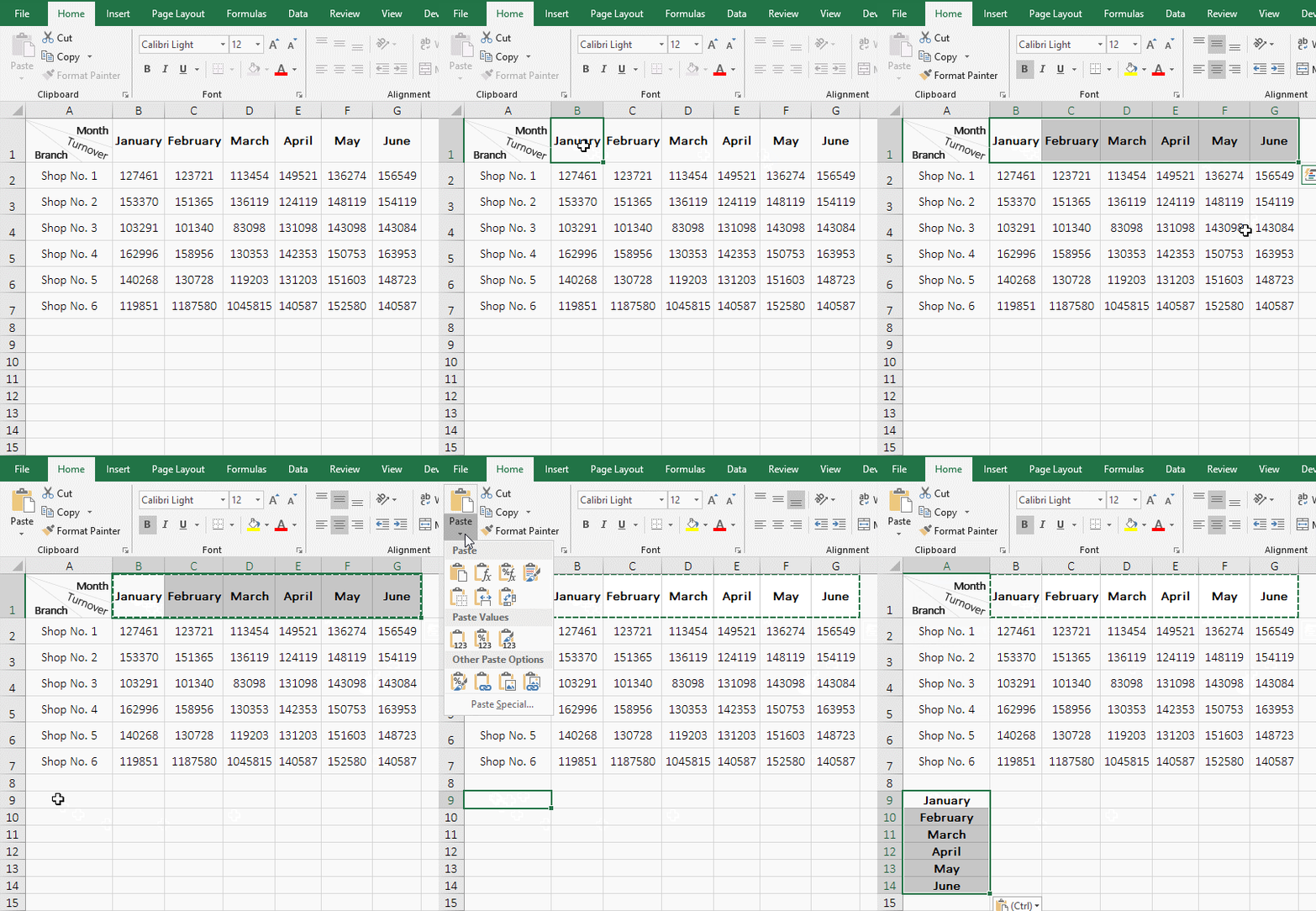
Figure 5
2. Insert the "Option Button" control.
A. Select the "Developer" tab, click "Insert", select "Option Button" in the pop-up controls, the mouse changes to a plus sign, move it to the position where you want to insert the "Option Button", and hold down the left button and drag to draw an option button, click the text inside to insert the cursor before the text, select all the text, and copy "Branch" into it;
B. Right-click the "Option Button", select "Format Control" from the pop-up options, open the "Format Control" dialog box, click the up arrow to the right of the "Cell Link" input box to shrink the dialog box, click B9, and it is the cell connected to the "Option Button", click "OK", and the "Option Button" is set;
C. Press Ctrl + C to copy the option button, then press Ctrl + V to paste it, align the pasted copy with the "Branch", click the text in the copy to position the cursor inside it, select all the text, and enter "Month"; Hold down Shift, right-click the" Branch "option button, select the two option buttons, then move them to the appropriate position, click any blank space to release the selected state of the option buttons, click "Branch", B9 displays 1 , Click "Month", B9 displays 2; the operation steps are shown in Figure 6:
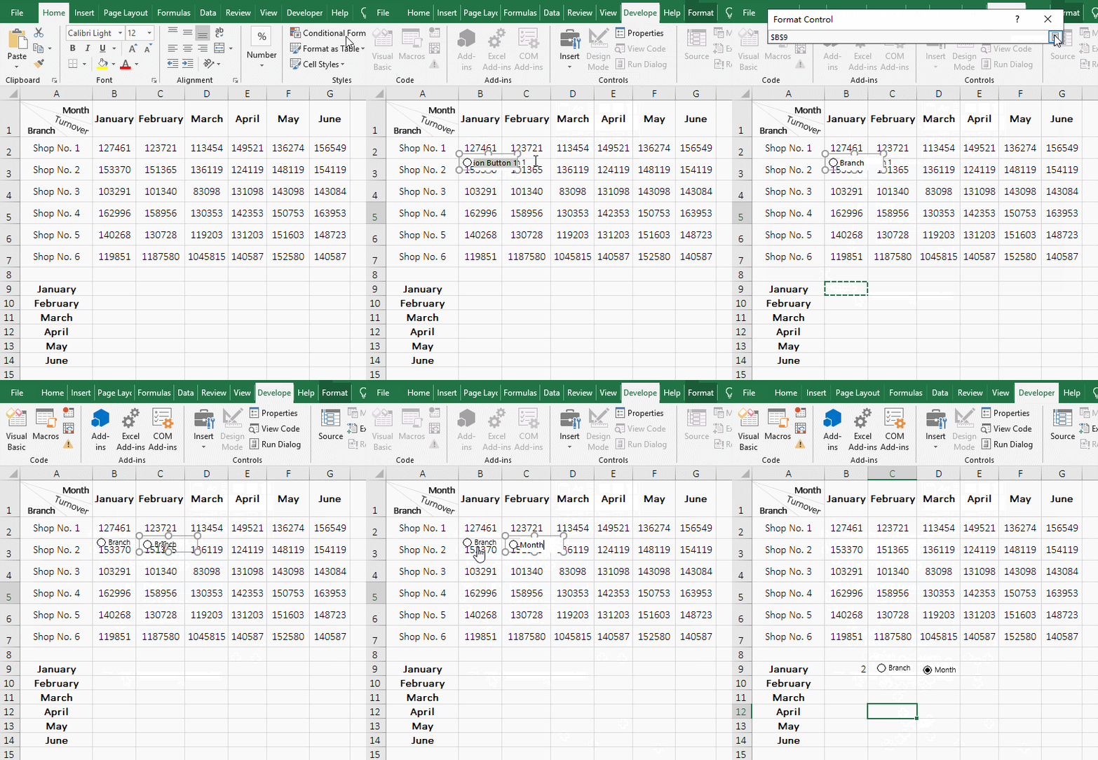
Figure 6
3. Add a reference to the option control with the "Definition name"
A. Right-click the "Branch" option button to select it, select the "Formula" tab, click "Define Name" to open the "New Name" dialog box; cope the "Categary_Options" to the right of "Name", select the text to the right of the equal sign(=) in the input box to the right of the "Refers to", enter IF(, click B9, enter "=1,", select A2:A7, enter ",", select A9:A14, enter ")", press Enter to confirm, the operation is complete. The demo is shown in Figure 7:
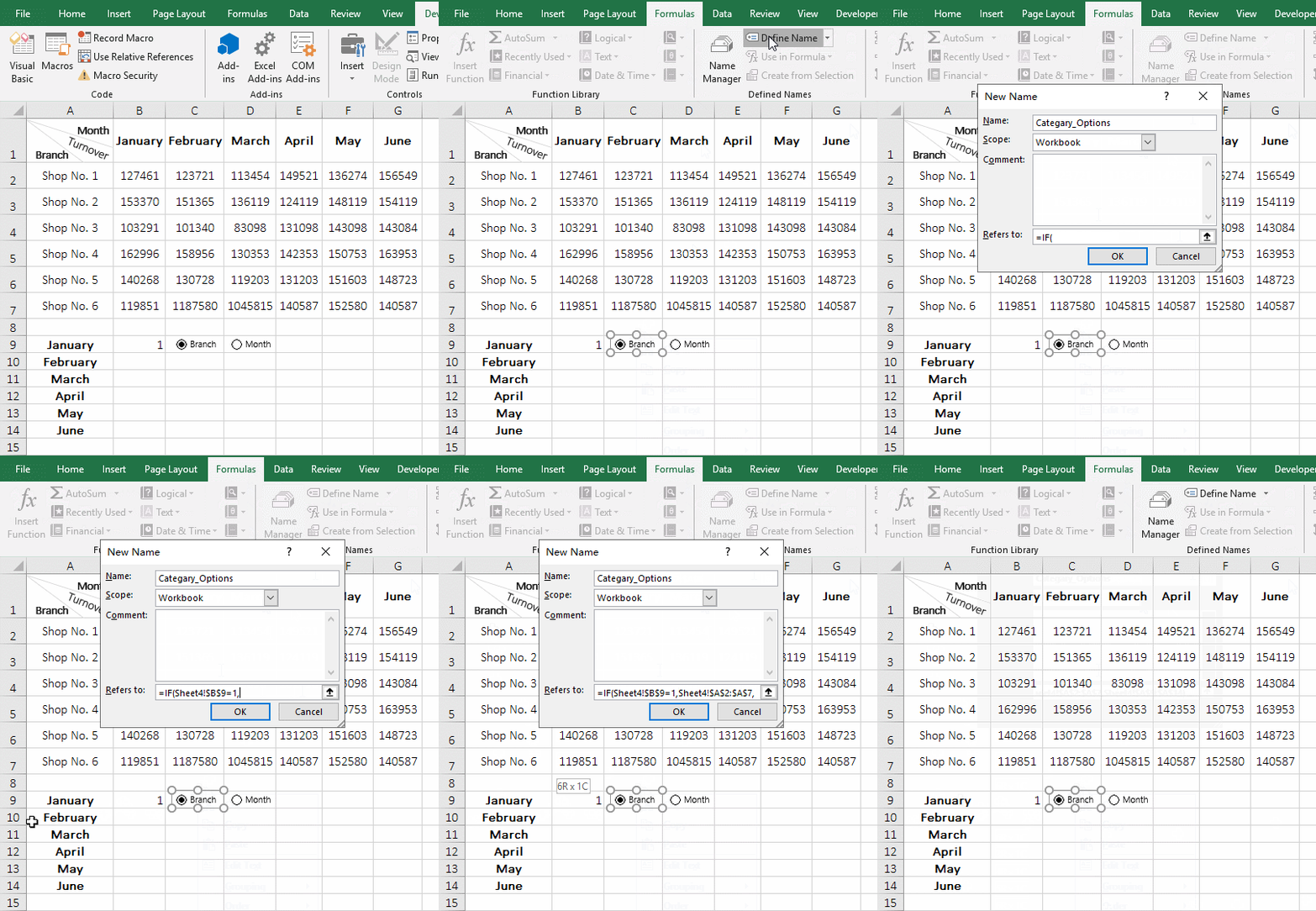
Figure 7
Hint: You can also directly copy the formula =IF(Sheet4!$B$9=1,Sheet4!$A$2:$A$7,Sheet4!$A$9:$A$14) into the input box to the right of "Refers to".
B. The formula =IF(Sheet4!$B$9=1,Sheet4!$A$2:$A$7,Sheet4!$A$9:$A$14) explanation:
The "Sheet4" is the name of the worksheet; Sheet4!$B$9=1 is the criteria of IF. If the criteria is satisfied, Sheet4!$A$2:$A$7 is returned, that is, all "Branch" are returned; otherwise Sheet4!$A$9:$A$14 is returned, that is, returns all "Months".
4. Insert a combo box control to achieve Excel chart dynamic range
A. Select the "Developer" tab, click "Insert", select "Combo Box" under "Form Controls", the mouse is changed to a plus sign, move it to the position where you want to insert the combo box, press the left button and drag to insert a combo box;
B. Right-click the "Combo Box", select "Format Control" from the pop-up options, open the "Format Control" dialog box. Copy the "Option Control" name "Categary_Options" defined in the previous step to the right of the "Input range"; click the up arrow to the right of the "Cell link" input box to shrink the dialog box, click C9 as the link cell of the combo box, and then click the up arrow to the right of the input box to expand the dialog box, click "OK";
C. Move the "combo box" to the right of "Month", click any blank space to release the selected state of the combo box, click "combo box", select the "Shop No. 3", then the "Shop No. 3" is its current option , the value in C9 becomes the corresponding value at the same time; select "Month", the combo box automatically changes to "March", click "Combine Box" again, and select "May"; the operation process steps, see screenshot in Figure 8:
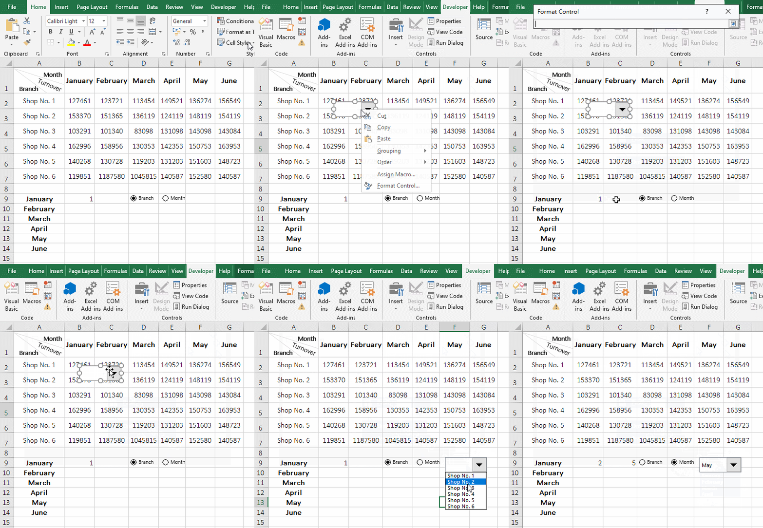
Figure 8
5. Define "X_axis_category" and "Dynamic_show_data" names.
A. Select the "Formulas" tab, click "Define Name" to open the "New Name" dialog, copy the "X_axis_category" into the input box to the right of the "Name", copy the formula =IF(Sheet4!$B$9=2,Sheet4!$A$2:$A$7,Sheet4!$A$9:$A$14) to the right of the "Refers to" and overwriting the original text, click "OK";
B. Click "Define Name" again, in the dialog box that has been opened, copy the "Dynamic_show_data" to the right of the "Name", copy the formula =IF(Sheet4!$B$9=1,OFFSET(Sheet4!$A$1,Sheet4!$C$9,1,1,6),OFFSET(Sheet4!$A$1,1,IF(Sheet4!$C$9<=6,Sheet4!$C$9,6),6,1)) to input box of the "Refers to" and cover the original text, click "OK"; two names are well defined; the operation steps, as shown in Figure 9:
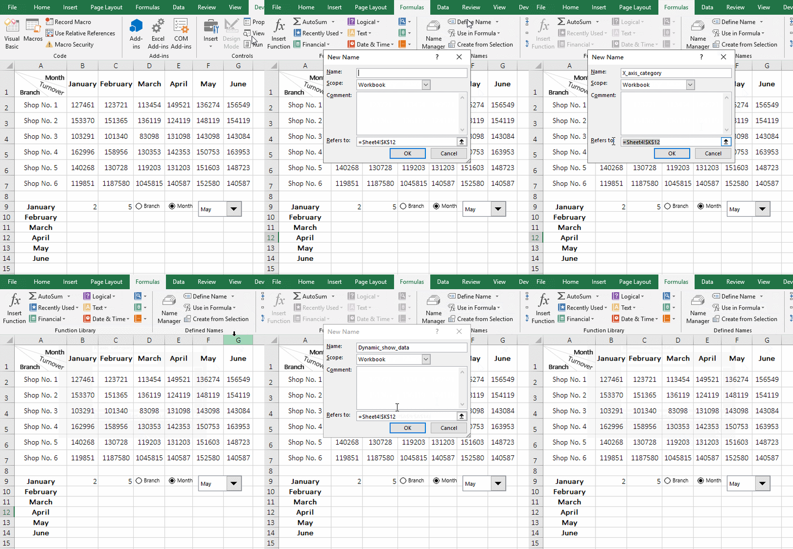
Figure 9
C. Formula description:
(1) =IF(Sheet4!$B$9=2,Sheet4!$A$2:$A$7,Sheet4!$A$9:$A$14) Means: If the value in B9 is 2, return the "Branch" in A2:A7," otherwise return the "Month" in A9:A14.
(2) =IF(Sheet4!$B$9=1,OFFSET(Sheet4!$A$1,Sheet4!$C$9,1,1,6), OFFSET(Sheet4!$A$1,1,IF(Sheet4!$C$9<=6,Sheet4!$C$9,6),6,1))
a. Sheet4!$B$9=1 is a criteria of IF, which means: if the value in B9 is equal to 1(that is, when "Branch" is selected), then execute OFFSET(Sheet4!$A$1,Sheet4!$C$9,1,1,6), that is, the monthly turnover of the currently selected "Branch" is displayed; otherwise execute OFFSET(Sheet4!$A$1,1,IF(Sheet4!$C$9<=6,Sheet4!$C$9,6),6,1), which shows the turnover of each store in the currently selected "Month".
b. OFFSET(Sheet4!$A$1,Sheet4!$C$9,1,1,6), $C$9 returns the selection value of "Combo Box", if the current selection value of "Combo Box" is "Shop No. 4", then $C$9 returns 4, and OFFSET returns the reference to cells rows 4 below A1 and column 1 to the right of A1 and height 1 and width 6, which returns $B$5:$G$5, that is, return to the monthly turnover of "Shop No. 4"(refer to the last step demo).
c. OFFSET(Sheet4!$A$1,1,IF(Sheet4!$C$9<=6,Sheet4!$C$9,6),6,1)
IF(Sheet4!$C$9<=6,Sheet4!$C$9,6) is used to return the column number, which means: if the value in C9 is less than or equal to 6, the value in C9 is returned, otherwise return 6, the main purpose is to prevent the selection value of the combo box from exceeding the number of columns in the table to be displayed in the chart(that is, 6 columns from "January" to "June");
If the current selection value of "Combo Box" is "April", then IF(Sheet4!$C$9<=6,Sheet4!$C$9,6) returns 4, and OFFSET(Sheet4!$A$1,1,IF(Sheet4!$C$9<=6,Sheet4!$C$9,6),6,1) becomes OFFSET (Sheet4!$A$1,1,4,6,1), which means: return to the reference to cells with row 1 under A1 and columns 4 to A1 and height 6 and width 1, that is, returns $E$2:$E$7, which is the turnover of each store in April.
6. Generate two-control dynamic chart.
A. Select the "Insert" tab, click the "Insert Column or Bar Chart" icon, and then select the first chart, then insert a blank chart. Drag the chart to an appropriate position, right-click the chart, and select "Send to Back" in the pop-up menu, put the chart at the bottom to show "option buttons and combo box";
B. Right-click the chart, and select "Select Data" from the pop-up menu to open the "Select Data Source" dialog box, click "Add", open the "Edit Series" dialog box, and select all text in the input box of "Series values", press Delete on the keyboard to delete them, click the sheet name "Sheet4", then copy the previously defined name "Dynamic_show_data" in the input box, and click "OK" to return to the "Select Data Source" dialog box;
C. Click "Edit" to open the "Axis Labels" dialog box, click on the sheet name "Sheet4", copy the name "X_axis_category" previously defined in the input box, click "OK" to return to the "Select Data Source" dialog box, click "OK" again, the chart is created; move the "Chart Title" to the left, clicks "Combo Box" and selects "Shop No. 3" to display the monthly turnover of "Shop No. 3"; selects "Month" to display the Turnover in "March", then select "May", then the turnover of each store in "May" will be displayed; the operation process steps are shown in Figure 10:
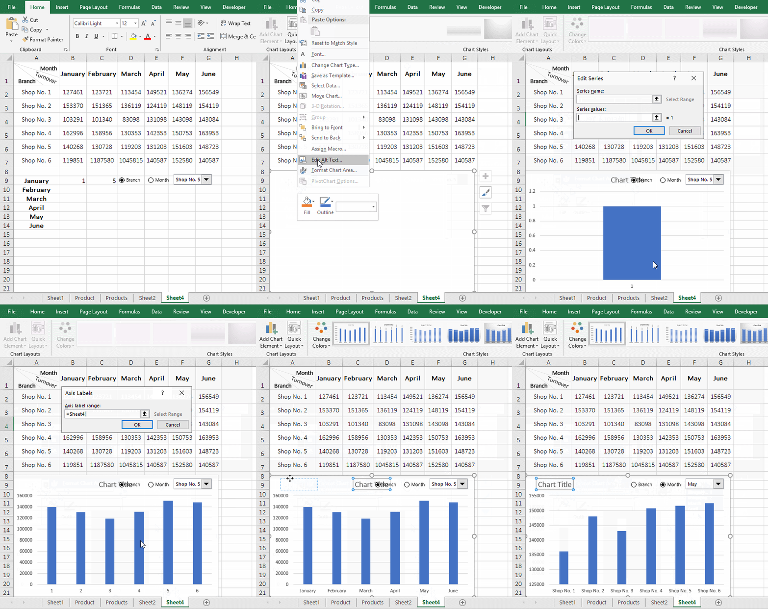
Figure 10
-
Related Reading
- How to move rows,columns,cells,table in excel(there
- How to subtotal in excel, with two fields, copy, sor
- Combine multiple excel sheets into one pivot table w
- How to create a pivot table in excel(15 examples, wi
- Excel pivot table percentage of grand total(parent r
- How to make a table of contents in word and change,
- How to convert excel to pdf(6 examples, with selecti
- How to make an excel spreadsheet, with the top 10 kn
- How to generate multiple reports from one pivot tabl
- How to use advanced filter in excel(7 examples, mult
- How to filter in excel(16 examples, with number,text
- Excel SumIf function with ?/*, Average and array mul